The Leiden Algorithm: How GraphRAG Finds Order Inside Knowledge Graphs

Introduction

GraphRAG starts from a simple problem: normal RAG is good at finding nearby chunks of text, but it often struggles when the answer depends on a bigger pattern spread across many documents. Instead of treating the corpus as only a pile of chunks, GraphRAG turns the text into a knowledge graph.

In that graph, entities become nodes, and relationships between entities become edges. But once the graph is built, it is usually too large and tangled to understand directly. This is where community detection becomes important as it helps in summarisation.

The Leiden algorithm is used for this step. It takes the knowledge graph and discovers communities inside it: clusters of entities that are more strongly connected to each other than to the rest of the graph.

Here is a clean schematic of how graphRAG works: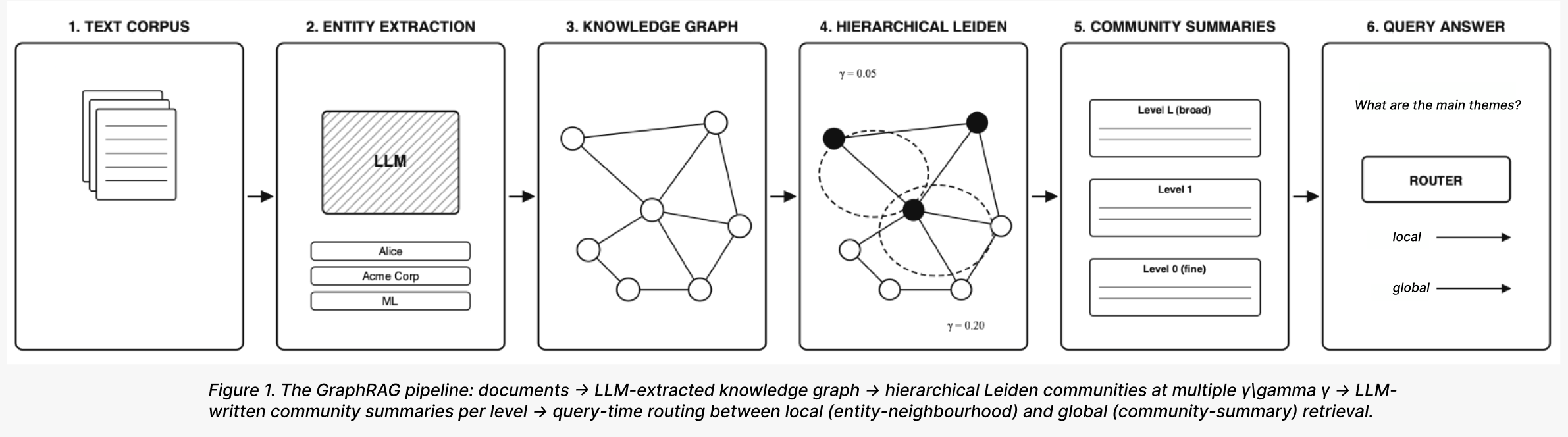

Why communities matter?

Networks are rarely random. People form friend circles, papers form research areas, videos form interest bubbles, and entities inside a knowledge graph form semantic neighborhoods. Community detection is useful because it gives us a way to discover these groups automatically.

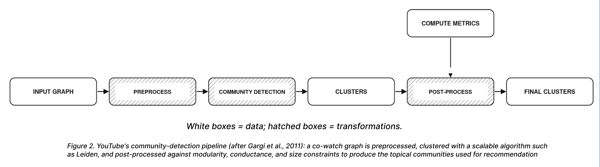
On YouTube, a viewer does not just watch isolated videos. Their clicks slowly reveal a sphere of interest, if we represent videos as nodes and similarities as edges, communities become recommendation neighborhoods.

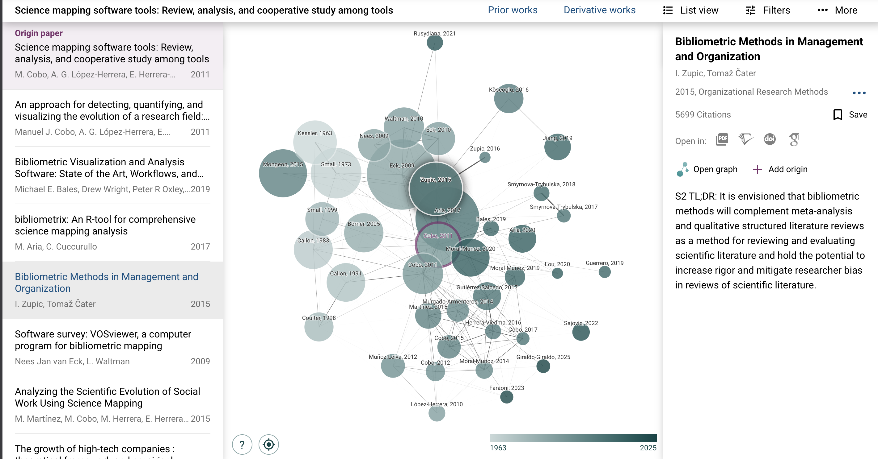
Connected Papers works in a similar spirit. A single paper is connected to nearby papers through citations, shared references, and semantic similarity. The graph around it naturally separates into research clusters: methods, applications and related fields

For GraphRAG, this becomes especially important. After documents are converted into a knowledge graph, the graph may contain thousands of entities and relationships. Leiden helps divide that graph into semantic clusters. Each cluster can then be summarized by an LLM, turning a messy knowledge graph into a layered map of meaning

Graph partitions and the combinatorial explosion

A graph is a set of nodes and edges:

$$G = (V, E)$$

where $V$ is the set of nodes and $E$ is the set of edges connecting them.

A partition divides the graph into communities:

$$C = \{C_1, C_2, \dots, C_k\}$$

Each node belongs to exactly one community.

For example:

$$C = \{\{0,1,2\},\{3,4,5,6,7\},\{8,9\}\}$$

This says nodes $0,1,2$ belong together, nodes $3,4,5,6,7$ belong together, and nodes $8,9$ form another group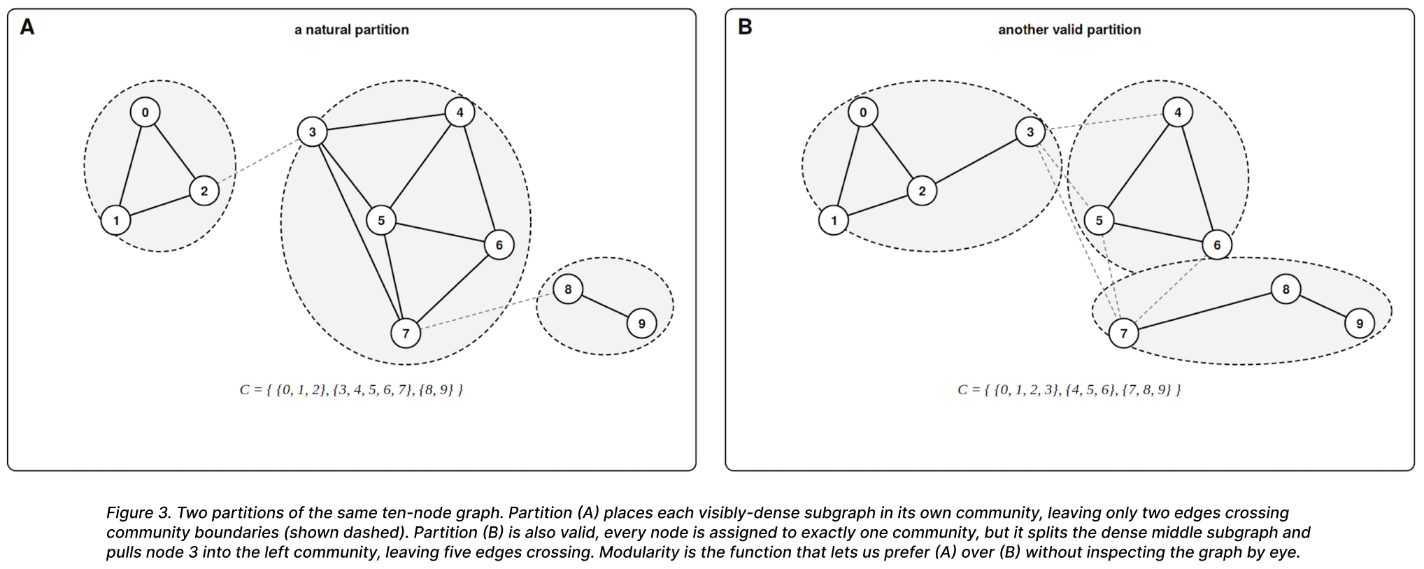

A partition is one possible way of saying: these nodes belong together

The hard part is not defining a partition. The hard part is choosing the best one. Even a tiny graph can be divided in many different ways. The above graph can also be partitioned in this way:

$$C = \{\{0,1,2\},\{3,4,5,6,7\},\{8,9\}\}$$

The first problem: Too many Partitions

Once we know what a partition is, the next question is:

How many possible ways can we divide a graph?

For a graph with $n$ nodes, the number of possible partitions is given by the Bell number:

$$B_{n+1}=\sum_{k=0}^{n}{n\choose k}B_k$$

and this grows extremely fast. For a graph with $n$ nodes, the number of possible partitions is given by the Bell number: | Nodes | Possible partitions | |——|——| | 1 | 1 | | 2 | 2 | | 3 | 5 | | 4 | 15 | | 5 | 52 | | 6 | 203 | | 7 | 877 | | 8 | 4140 | | 9 | 21147 | | 10 | 115975 |

So even before we talk about a large knowledge graph, brute force is already failing

For GraphRAG, this matters because a knowledge graph may contain thousands of entities. Trying every possible grouping is impossible. Hence, we need a smarter way to search

The second problem: What makes a parition good?

A first attempt might be simple:

$$\text{Score}= \frac{\text{edges inside communities}} {\text{total edges}}$$ If most edges stay inside communities rather than crossing between them, the partition probably captures some meaningful structure in the graph. But this definition is still informal. To make it precise, we need a mathematical way to count how many edges remain inside a community. So let us simplify the fraction and derive it step by step

Consider a graph (G) with:

$$|V(G)| = n$$

nodes and

$$|E(G)| = m$$

edges.

We represent the graph using the adjacency matrix:

$$A_{uv}= \begin{cases} 1 & \text{if } u \text{ and } v \text{ are connected} \\ 0 & \text{otherwise} \end{cases}$$

Now suppose we focus on a single community $c$. To count the edges that remain inside this community, we sum over every pair of nodes belonging to $c$:

$$\sum_{u\in c}\sum_{v\in c} A_{uv}$$

This quantity counts all internal connections of the community. To convert this into a fraction of all edges in the graph, we divide by the total number of edge appearances. Since the graph is undirected:

$$A_{uv}=A_{vu}$$

every edge appears twice in the adjacency matrix. So the fraction of edges inside community $c$ becomes:

$$e_c= \frac{1}{2m} \sum_{u\in c}\sum_{v\in c} A_{uv}$$

But there is a problem. If we put every node into one giant community, then every edge becomes an internal edge: $$\text{score}=1$$ So the naive score says the best partition is: $$C=\{V\}$$

One giant community, and that is useless because large communities naturally contain many internal edges simply because they are large. So the real question becomes:

Are there more internal edges than we would expect by chance?

That question leads us to modularity. >Questions to ponder: 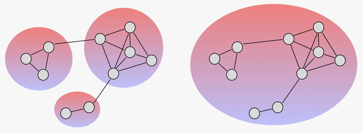> Which one is actually more meaningful? > Even though the second has score (1.00), it tells us nothing, hence a score that rewards only internal edges will always prefer one giant community.

Mark Newman’s key insight was that a good community structure is not simply one with many edges inside communities. That can happen just because the communities are large. A good partition should have more internal structure than we would expect by chance > 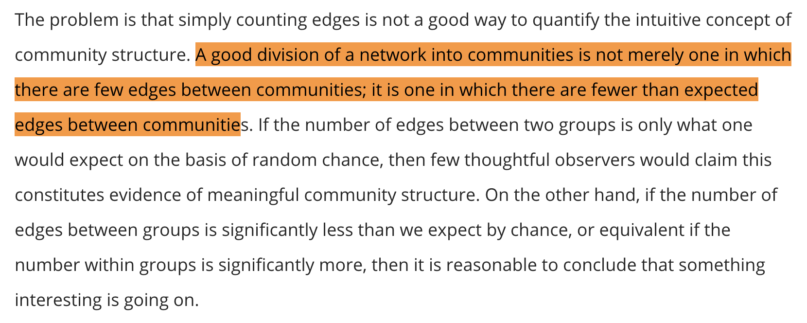This changes the problem.

We are no longer asking:

$$\text{How many edges are inside the communities?}$$

We are asking: $$\text{How surprising is this partition compared to random wiring?}$$

That difference is subtle, but extremely important. A good partition is not just one with many internal edges. A good partition has more internal structure than we would expect to appear by chance alone.

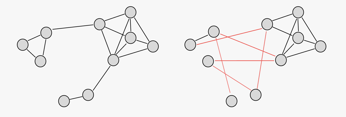
View	Meaning
Actual graph (On the Left)	What we observed
Random baseline (On the Right)	What we would expect by chance

Now the question arises how do we define a good baseline? As we cannot compare against just any random graph. A totally random graph might change the number of edges or make high-degree nodes look ordinary. That would not be fair. So our random baseline must preserve the important properties of the original graph:

$$n = \text{number of nodes}$$

$$m = \text{number of edges}$$

$$k_v = \text{degree of each node}$$ # The configuration model and the random baseline

To know whether a community is meaningful, we must compare the graph against a fair random baseline. But the random graph cannot be completely arbitrary. It must preserve the important structural properties of the original graph:

$$n = \text{number of nodes}$$

$$m = \text{number of edges}$$

$$k_v = \text{degree of node } v$$

Otherwise the comparison would not be fair. A graph with completely different degree distributions would naturally produce different connectivity patterns. So instead of comparing against random wiring alone, we compare against a random graph that preserves the degree of every node. This leads us to the configuration model, also called the degree-preserving random graph.

The Stub Model

Imagine cutting every edge in half. Each half-edge is called a stub. If a node has degree $k_v$, then it owns exactly $k_v$ stubs.

So:

• a node with degree $5$ has $5$ stubs
• a node with degree $2$ has $2$ stubs

We now reconnect these stubs randomly.The resulting graph has:

• the same number of nodes
• the same number of edges
• the same degree sequence

but different wiring. So high-degree nodes remain high-degree, and low-degree nodes remain low-degree.

Expected Connections in the Random Graph

Now suppose we want to know:

How many edges would we expect between two nodes purely by chance?

Consider two nodes: $u$ and $v$. Node $u$ has degree: $k_u$ and node $v$ has degree: $k_v$

This means:

• node $u$ owns $k_u$ stubs
• node $v$ owns $k_v$ stubs

Since every edge contributes two stubs, the graph contains: $2m$ total stubs. Now pick one stub from node (u). There are: 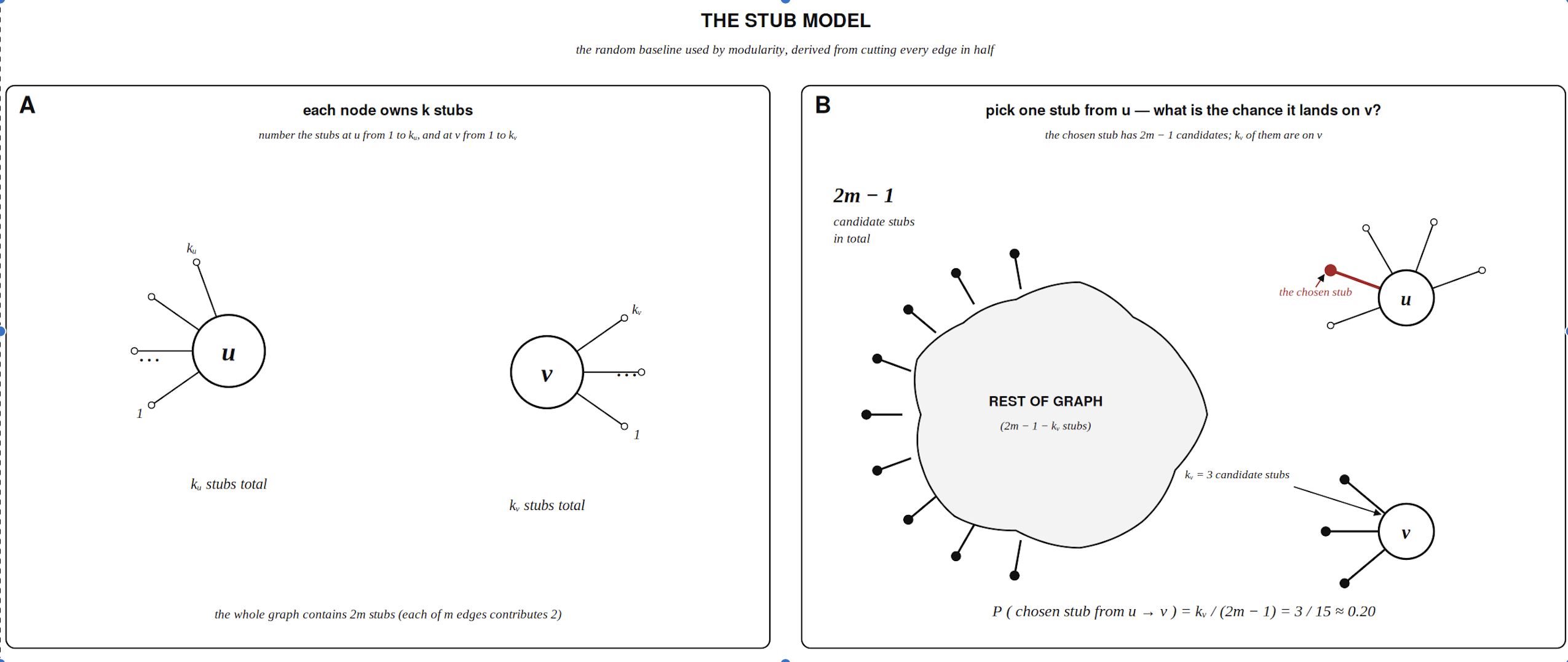$2m-1$

possible stubs it could connect to. Out of those, exactly (k_v) belong to node (v). So the probability that one stub from (u) connects to node (v) is:

$$\frac{k_v}{2m-1}$$

But node $u$ has $k_u$ opportunities to make such a connection. So the expected number of connections between $u$ and $v$ becomes:

$$\mathbb{E}[A_{uv}] = \frac{k_u k_v}{2m - 1}$$ which simplifies to:

$$\mathbb{E}[A_{uv}] = \frac{k_u k_v}{2m-1}$$

PS: a more formal proof exists and for those who are interested here it is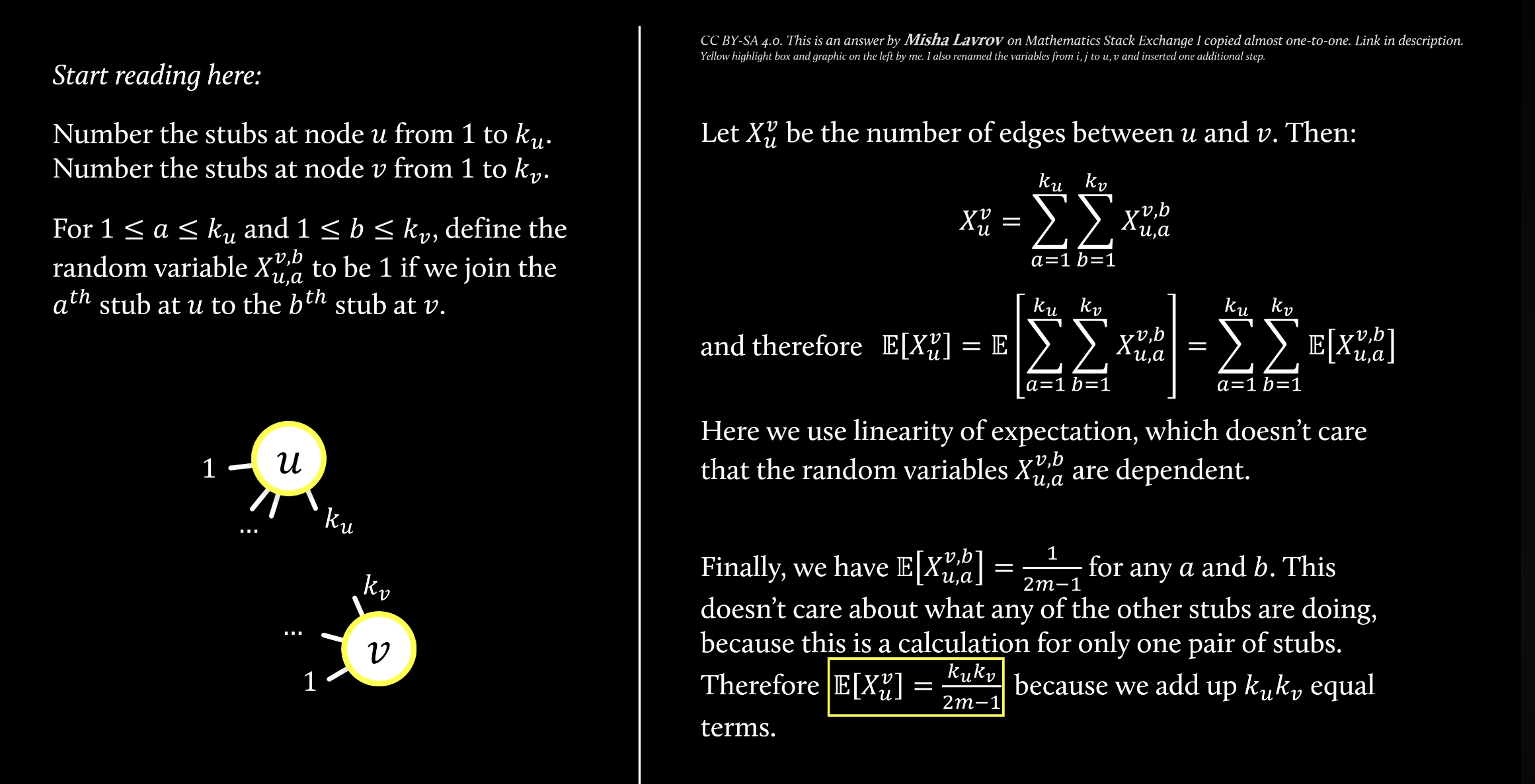

Why This Matters

This term becomes the random baseline inside modularity.

It tells us:

how many edges we would expect to see between two nodes purely because of their degrees.

This is extremely important. If two nodes both have very large degree, they are already likely to connect by chance. So modularity should not reward an edge simply because it exists.Instead, modularity rewards edges that appear more often than the degree-preserving random graph would predict.

From Internal Edges to Modularity

Earlier, we defined the fraction of edges inside a community (c) as:

$$e_c= \frac{1}{2m} \sum_{u\in c} \sum_{v\in c} A_{uv}$$

Now we can compute the expected fraction of such edges in the random graph. Replacing $A_{uv}$ with its expected value gives:

$$a_c^2 = \frac{1}{2m} \sum_{u\in c} \sum_{v\in c} \frac{k_u k_v}{2m}$$

where:

$$a_c = \frac{1}{2m} \sum_{v\in c} k_v$$

represents the fraction of all edge stubs attached to community $c$

• $e_c$ measures the actual internal connectivity
• $a_c^2$ measures the expected connectivity under random wiring

The difference between them gives the true community signal.

View	Meaning
Actual graph	What we observed
Random baseline	What we would expect by chance
Difference	The community signal

This finally leads us to modularity:

$$Q(C) = \sum_{c\in C} \left( e_c-a_c^2 \right)$$

or equivalently: $$Q(C)=\frac{1}{2m}\sum_{c\in C}\sum_{u\in c}\sum_{v\in c}\left(A_{uv}-\frac{k_u k_v}{2m}\right)$$ This is the central idea behind modularity:

A community is meaningful when it contains more internal structure than we would expect from random wiring alone.

From modularity to optimisation: the Louvain algorithm

We now have a precise quality function:

$$Q(C)=\frac{1}{2m}\sum_{c\in C}\sum_{u\in c}\sum_{v\in c}\left(A_{uv}-\frac{k_u k_v}{2m}\right)$$

But knowing how to score a partition does not yet tell us how to find a good one. There are $B_n$ partitions of an $n$-node graph (Bell numbers), and we already saw this grows faster than any algorithm can enumerate. We need a heuristic that climbs $Q$ without examining every partition. The Louvain algorithm was, for a decade, the standard answer. Its design is elegant, it proceeds in two phases.

Phase 1: Local moving

Start with every node in its own community. Then repeat until nothing changes:

For each node (i), compute the change in modularity $Delta Q$ for moving $i$ into each neighbouring community. Move $i$ to the community that maximises $Delta Q$ (and only if $Delta Q > 0$ )

For an isolated node (i) being placed into community (C), the move-gain formula is:

$$\Delta Q_{i\to C} \;=\; \frac{1}{2m}\left[\,2\,k_{i,C} \;-\; \frac{k_i \cdot \Sigma_{\text{tot}}(C)}{m}\,\right]$$

where:

• $k_{i,C}=\sum_{v\in C} A_{iv}$ is the total edge weight from $i$ into $C$,
• $\Sigma_{\text{tot}}(C)=\sum_{v\in C}k_v$ is the total degree of community $C$, and
• $k_i$ is the degree of $i$.

The intuition splits cleanly into two terms:

$$\frac{2k_{i,C}}{2m}$$

is the observed coupling between $i$ and $C$, and

$$\frac{k_i\,\Sigma_{\text{tot}}(C)}{2m^2}$$

is the expected coupling under the configuration null model. We move $i$ into $C$ iff observed exceeds expected by the most.

Phase 2: Aggregation

Once no node wants to move, collapse each community into a single super-node. Edges between communities become weighted edges between super-nodes; edges within a community become self-loops on the super-node. The aggregated graph $G'$ is much smaller, but its modularity is identical to that of the partition we just found on $G$.

Run Phase 1 again on $G'$. And again. The algorithm terminates when neither phase produces any change. This greedy hill-climb is fast $O(m \log n)$ per pass in practice) and finds partitions whose modularity is, on most networks, within a few percent of the global optimum.

But it has a problem! ## Why Louvain Isn’t Enough: the Disconnected-Communities Bug

The problem is subtle, and for ten years almost everyone using Louvain failed to notice it. Then in 2019, Traag, Waltman & van Eck proved something embarrassing:

Louvain’s communities are not guaranteed to be connected. A “community” returned by Louvain may consist of two or more disconnected pieces of the original graph.

This is not a numerical artefact. It happens routinely on real networks, and the disconnection can be arbitrarily severe.

A minimal example

Consider a community (C={a,b,c,d,e,f}) inside some larger graph, structured as two triangles bridged by a single node:

$$\underbrace{a-b-c-a}_{\text{triangle }T_1}\;,\quad \underbrace{d-e-f-d}_{\text{triangle }T_2}\;,\quad b-d \text{ is the only edge connecting } T_1 \text{ and } T_2.$$

Within (C), node (b) is the only path between ({a,c}) and ({d,e,f}). Now suppose (b) also has strong external ties to some neighbouring community (C’), strong enough that:

$$\Delta Q_{b \to C'} \;>\; 0.$$

Louvain dutifully moves $b$ out of $C$ and into $C'$. The remaining community {$C$ - $b$} = {a,c,d,e,f}) is still labelled the same community, but it is now disconnected: there is no path from $a$ to $d$ using only nodes in $C$.

The crucial observation: at no point during Phase 1 does Louvain check connectivity. Modularity only cares about edge counts and degree expectations; it has no opinion on whether a community is one piece or many.

Why this matters for GraphRAG

If a knowledge-graph community is disconnected, the LLM summary of that community will try to compress two unrelated semantic regions into one description. The resulting “community summary” is incoherent at best and hallucinatory at worst. For systems that rely on hierarchical community summaries like GraphRAG this failure mode silently degrades retrieval quality without producing any obvious error signal. This is precisely the gap the Leiden algorithm was designed to close.

The Leiden Algorithm: Local Move → Refinement → Aggregation

Leiden keeps Louvain’s overall structure but inserts a refinement step between local moving and aggregation. The full algorithm has three phases:

1. Fast local moving: like Louvain’s Phase 1, but only re-visits nodes whose neighbourhood has changed (a significant speedup).
2. Refinement: within each community found in step 1, run a constrained local move that can only place nodes into sub-communities of their current community. This step is what guarantees connectedness.
3. Aggregation: collapse the graph based on the refined partition (preserving well-connectedness), but initialise the next iteration’s communities using the membership from the unrefined partition (preserving the global structure step 1 found). ### Phase 2 in detail: refinement

This is the heart of the algorithm.

Let $P$ be the partition produced by Phase 1. For each community $C \in P$, Leiden temporarily breaks the community apart and re-initializes every node inside $C$ as its own singleton community.

The algorithm then iterates over nodes $i \in C$ and considers merging $i$ into a candidate sub-community $S \subseteq C$, but only if two conditions hold:

• Locality: the merge must remain inside the original community $C$,
• Well-connectedness: the candidate sub-community must remain sufficiently connected to the rest of $C$.

Formally, Leiden requires:

$$E(S,C-S)\geq \gamma |S||C-S|$$

where $E(S,C-S)$ denotes the total edge weight between $S$ and the rest of the community, and $\gamma$ controls how strongly connected the partition must remain.

Among all valid merges, Leiden does not choose greedily. Instead, it samples a merge with probability proportional to:

$$\exp(\Delta Q / \theta)$$

where $\Delta Q$ is the modularity gain and $\theta$ is a small temperature parameter. This randomness is intentional. Purely greedy optimization tends to lock in early decisions and miss better local refinements, while probabilistic selection allows Leiden to explore more of the nearby partition landscape before aggregation.

Why this fixes Louvain’s bug

Crucially, after refinement, every refined sub-community is by construction internally connected, it was built by merging singletons under a well-connectedness rule, so disconnection is impossible. When we then aggregate, the super-nodes correspond to refined sub-communities, not to the original Louvain communities. The disconnected-community failure mode cannot survive into the aggregated graph.

Guarantees

Traag et al. prove that the Leiden algorithm satisfies a hierarchy of guarantees that Louvain does not:

Property	Louvain	Leiden
All communities connected after each iteration	No	Yes
$\gamma$-separation after each iteration	No	Yes
$\gamma$-connectedness after each iteration	No	Yes
Node-optimal assignment after stable iteration	Partial	Yes
Subset-optimal (every subset optimally placed) asymptotically	No	Yes
Uniform $\gamma$-density asymptotically	No	Yes

Empirically, Leiden is also typically faster than Louvain on the same graph, because the fast local-move phase avoids re-examining nodes whose neighbourhoods did not change.

Pseudocode

Input:  graph G = (V, E, w), quality function Q
Output: partition P of V
 
P ← singleton partition of V        // every node in its own community
repeat:
    P ← FastLocalMove(P, G, Q)      // Phase 1
    if P is singleton: stop
    P_refined ← Refine(P, G, Q)     // Phase 2 — the new step
    G ← Aggregate(G, P_refined)     // Phase 3
    P ← lift(P, P_refined)          // use original P's membership
                                      // on the aggregated graph
until no improvement
return P

The line lift(P, P_refined) is the conceptual twist that often trips people up: we aggregate by the refined sub-communities (to lock in connectedness), but we re-initialise the next iteration’s community labels using the original Phase-1 communities (to preserve the global structure already discovered).

Worked Example: A Five-Node Leiden Walkthrough

Now that we understand modularity, we can finally watch a real community detection algorithm work step by step. Instead of discussing the algorithm abstractly, we will follow a small graph and observe how communities emerge through local modularity optimization.

This is the core intuition behind the Leiden algorithm.

The Graph

We begin with a weighted graph containing five nodes.

The graph has:

$$m=15 \quad\Rightarrow\quad 2m=30$$

The node degrees are:

$$k_0=5,\quad k_1=6,\quad k_2=8,\quad k_3=5,\quad k_4=6$$

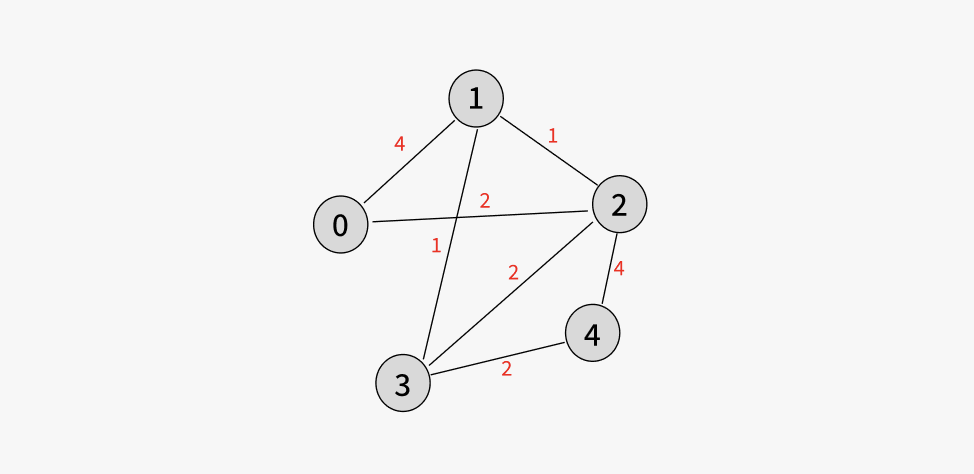
The weighted edges are:

$$A_{0,1}=4$$

$$A_{0,2}=1$$

$$A_{1,2}=1$$

$$A_{1,3}=1$$

$$A_{2,3}=2$$

$$A_{2,4}=4$$

$$A_{3,4}=2$$

Initially, every node starts in its own community:

$$C=\{\{0\},\{1\},\{2\},\{3\},\{4\}\}$$

The algorithm now asks:

Which local move increases modularity the most?

Step 1: Node 2 Chooses a Community

Suppose node (2) evaluates its neighboring communities.

It computes the modularity gain obtained by joining each neighboring node.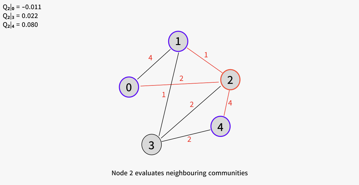

Option 1: Join Node 0

$$Q_{2|0}= \frac{1}{30} \left(1-\frac{8\cdot5}{30}\right) = -0.011$$

This move produces negative gain.

So joining node (0) is not attractive.

Option 2: Join Node 3

$$Q_{2|3} = \frac{1}{30} \left(2-\frac{8\cdot5}{30} \right) = 0.022$$

This is better.

The observed edge weight exceeds the random expectation slightly.

Option 3: Join Node 4

$$Q_{2|4} = \frac{1}{30} \left( 4- \frac{8\cdot6}{30} \right) = 0.080$$

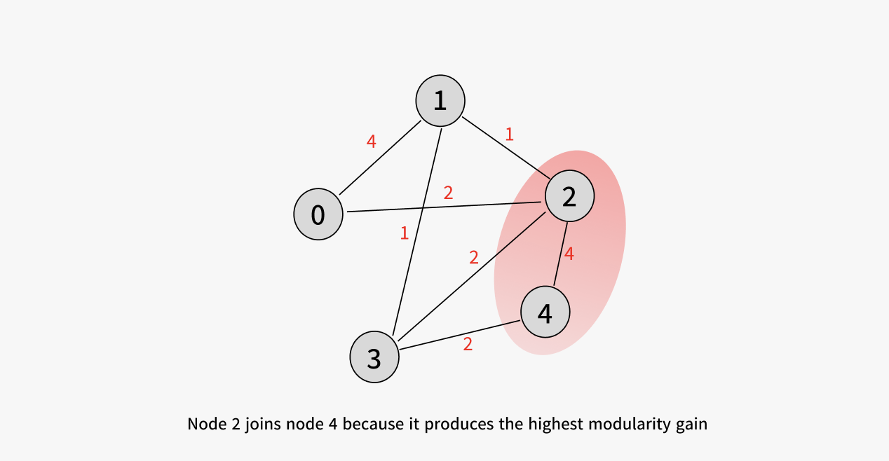
This gives the highest gain.

The connection between nodes (2) and (4) is much stronger than random chance would predict.

So Leiden chooses:

$$2 \rightarrow 4$$

The partition now becomes:

$$C=\{\{0\},\{1\},\{2,4\},\{3\}\}$$

Step 2: Node 0 Evaluates Its Neighbors

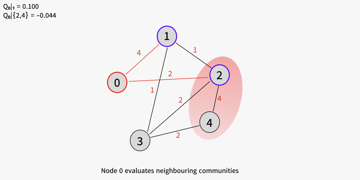
Now node (0) considers possible moves. The strongest neighboring community is node (1)

The modularity gain becomes:

$$Q_{0|1} = \frac{1}{30} \left( 4-\frac{5\cdot6}{30} \right) = 0.100$$

Node (0) could also consider joining the community:

$$\{2,4\}$$

Notice that after node (2) joins node (4), the algorithm no longer evaluates node (2) individually. It evaluates the entire community.

The total degree of the community becomes:

$$k_2+k_4 = 8+6 = 14$$

Node (0) has only one connection into this community:

$$A_{0,2}=1\quad\text{and}\quad A_{0,4}=0$$

So the modularity gain becomes:

$$Q_{0|\{2,4\}} = \frac{1}{30} \left( 1-\frac{5\cdot14}{30} \right) = -0.044$$

This is negative.

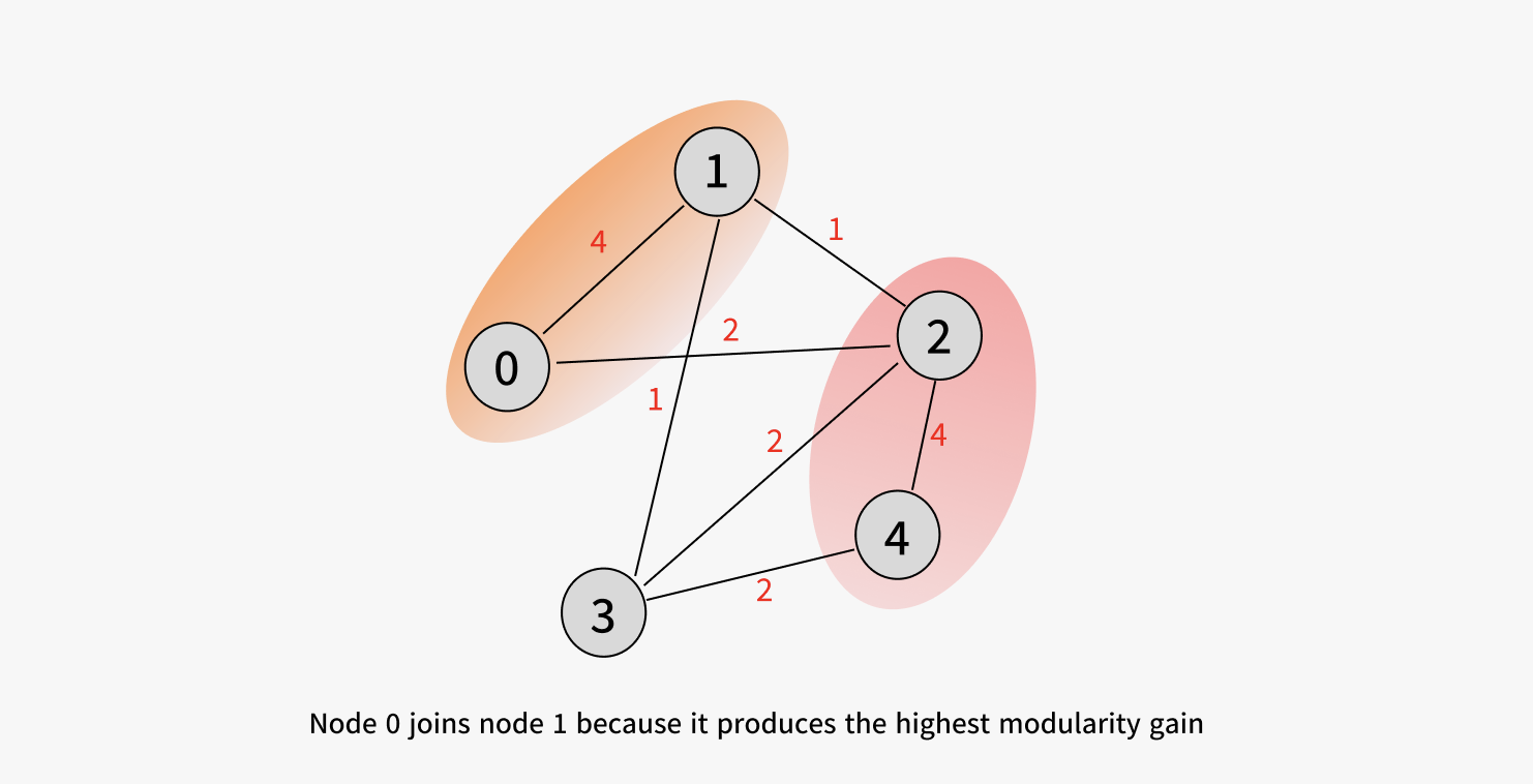
Even though node (0) is connected to node (2), the connection is not strong enough compared to what random chance already predicts from the large degree of the community.

So node (0) prefers joining node (1). The partition becomes:

$$C=\{\{0,1\},\{2,4\},\{3\}\}$$

Step 3: Node 3 Decides

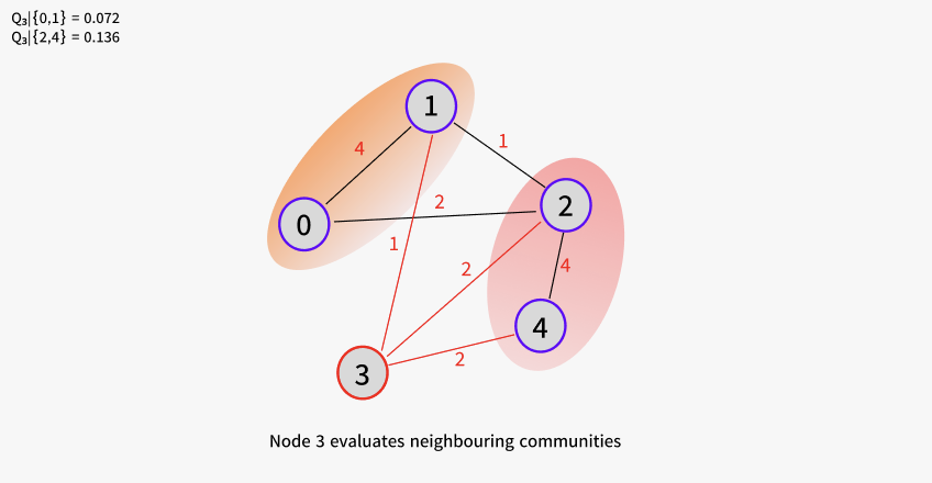
Now node (3) must decide where it belongs.

There are two candidate communities:

• the community containing (0) and (1)
• the community containing (2) and (4)

Option 1: Join ({0,1})

$$Q_{3|1|0} = 0.000 - 0.028 + 0.100 = 0.072$$

Option 2: Join ({2,4})

$$Q_{3|2|4} = 0.022 + 0.033 + 0.080 = 0.136$$

The second option gives a larger modularity gain.

So node (3) joins the community containing nodes (2) and (4).

The final local partition becomes:

$$C=\{\{0,1\},\{2,3,4\}\}$$

At this point, the graph has separated naturally into two dense regions.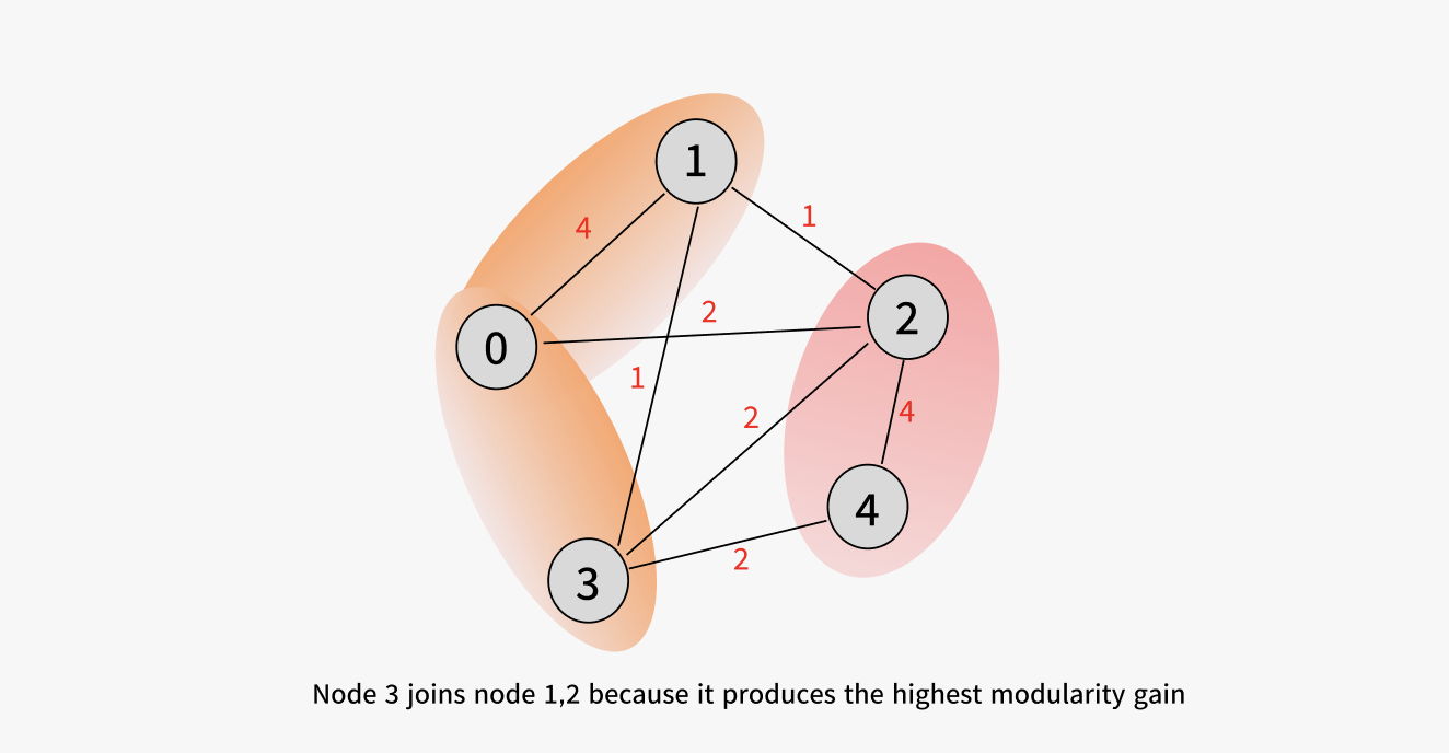

A small auxiliary example where refinement matters

To see refinement actually do work, consider a graph designed to trip Louvain up. Let:

• Nodes: $\{a, b, c, d, e, f\}$ plus an external node $x$.
• Edges (all weight 1 unless noted):
  • Triangle 1: $a-b$, $b-c$, $a-c$
  • Triangle 2: $d-e$, $e-f$, $d-f$
  • Single bridge: $b-d$
  • Strong external pull: $b-x$ with weight 3, and $x$ is in some external community $C'$ of total degree $\sim 6$.

Louvain’s Phase 1 will likely first place all six nodes into one community $C=\{a,b,c,d,e,f\}$ because the intra-community edges outnumber the external ones. Then it revisits $b$ and, because of the strong $b-x$ tie, computes $\Delta Q_{b\to C'} > 0$ and moves $b$ out. The resulting “community” $\{a,c,d,e,f\}$ is disconnected: removing $b$ severed the only $T_1$–$T_2$ link.

Now run refinement on this Louvain output. Inside $\{a,c,d,e,f\}$:

• Sub-singletons: $\{a\}, \{c\}, \{d\}, \{e\}, \{f\}$.
• The well-connectedness check between $\{a,c\}$ and $\{d,e,f\}$ requires an edge between them. There is none (the only such edge was $b-d$, and $b$ left).
• Therefore the refinement cannot merge $\{a,c\}$ with $\{d,e,f\}$. The refined sub-communities remain split: $\{a,c\}$ and $\{d,e,f\}$.

When we aggregate, the super-node for “old community $C\setminus\{b\}$” is replaced by two super-nodes, one for $\{a,c\}$, one for $\{d,e,f\}$. The disconnection is fixed before the next iteration. Leiden does in one pass what Louvain cannot do in any number of passes.

Beyond Modularity: the Resolution Limit and CPM

Everything we have built so far rests on optimising modularity. But modularity has a well-known structural defect that becomes important the moment your graph is large, which it always is in GraphRAG.

The resolution limit

Fortunato and Barthélemy (2007) proved that modularity-maximising algorithms cannot detect communities smaller than roughly $\sqrt{2m}$ edges, regardless of how clearly defined those communities are.

The intuition is in the formula. Recall:

$$Q(C)=\frac{1}{2m}\sum_{c\in C}\left(\Sigma_c - \frac{\Sigma_{\hat{c}}^2}{2m}\right)$$

The expected-edge term scales like $\Sigma_{\hat{c}}^2/(2m)$. For small communities, this expectation is tiny, and a small constant modularity gain from merging two small communities can dominate the loss from doing so — even when those communities are otherwise clearly distinct.

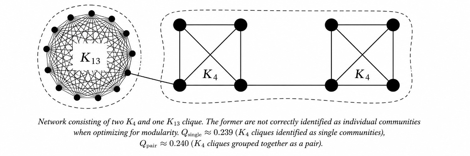
The canonical counter-example is a graph composed of three pieces: two complete graphs $K_4$ (each with $\binom{4}{2}=6$ edges) joined by a single bridge edge, and a much larger clique $K_{13}$ with $\binom{13}{2}=78$ edges, plus an arbitrary graph providing the remaining edges. The total edge count satisfies $(m \approx 98)$. The condition

$$m_c \;<\; m/2 \quad\Longleftrightarrow\quad 6 < 49$$

is comfortably met for each (K_4). And indeed: modularity-maximisation on this graph groups the two (K_4)s into a single community, even though they are visibly two distinct cliques connected by one edge. Computing both partitions:

• $Q_{\text{single}} \approx 0.239$, each $K_4$ forms its own community.

• $Q_{\text{pair}} \approx 0.240$, the two $K_4$ graphs are merged into one larger community.

Modularity therefore prefers the wrong partition by a tiny margin. The important point is that this is not an implementation bug. It is a limitation of modularity itself. As the graph grows larger, the problem becomes worse. Small communities become increasingly invisible relative to the total graph size. For a knowledge graph with:

$$m \sim 10^6$$

modularity cannot reliably detect communities much smaller than:

$$\sqrt{2 \cdot 10^6} \approx 1400$$

edges. Any meaningful cluster smaller than this scale may be absorbed into a larger neighboring community.

CPM: the Constant Potts Model

The cleanest answer to the resolution limit is to abandon modularity’s expected-edge term entirely and replace it with a resolution parameter $\gamma$ that has a clean interpretation. The Constant Potts Model (Traag, Van Dooren & Nesterov, 2011) is defined by:

$$H_{\text{CPM}}(C) \;=\; -\sum_{c\in C}\!\left[\, e_c \;-\; \gamma \binom{n_c}{2} \,\right]$$

where:

• $e_c$ is the number of internal edges of community $c$,
• $n_c$ is the number of nodes in $c$, and
• $\gamma \in [0,1]$ is the resolution parameter.

The negative sign is so that minimising $H_{\text{CPM}}$ is equivalent to maximising the quantity in brackets. The bracket has a clean meaning: a community contributes positively iff its internal edge density exceeds $\gamma$.

In fact, one can show that any optimal CPM partition satisfies:

$$\text{internal density of } c \;>\; \gamma \;>\; \text{density between } c \text{ and any other community.}$$

So $\gamma$ is a literal density threshold, controlled by the user. There is no resolution limit — communities of any size can be detected, provided their density exceeds $\gamma$. Smaller $\gamma$ gives coarser communities; larger $\gamma$ gives finer ones, with a strictly nested hierarchy as $\gamma$ sweeps over its range.

When to use which

Property	Modularity	CPM
Resolution limit	Yes ($\sqrt{2m}$)	No
Resolution parameter	None (fixed null model)	$\gamma$ tunable
Works with negative edge weights	No	Yes
Natural hierarchy	No	Yes, sweep $\gamma$
Default in leidenalg	Yes	Available
Used by Microsoft GraphRAG	No	Yes

For small social networks and the karate-club-scale demonstrations that fill most textbooks, modularity is fine. For knowledge graphs with thousands or millions of entities, CPM is the appropriate quality function, and it is what production GraphRAG implementations actually use.

How GraphRAG Uses Hierarchical Leiden

GraphRAG does not use Leiden as a single clustering step. Instead, it runs Leiden with CPM across multiple resolutions to build a hierarchy of communities.

Documents are first converted into a knowledge graph:

$$G=(V,E)$$

using entity and relationship extraction. Leiden then produces a nested sequence of partitions:

$$P_0 \succ P_1 \succ \cdots \succ P_L$$

where finer communities merge into progressively coarser ones.

LLMs summarize communities at every level, creating a hierarchy of semantic summaries. At query time, GraphRAG can either retrieve locally through neighborhood traversal or globally by reasoning over higher-level community summaries.

This hierarchical structure is what allows GraphRAG to move between fine-grained details and corpus-level themes efficiently.

Why Leiden specifically

The hierarchy is only as reliable as its communities. If a community is disconnected, the LLM is forced to summarize unrelated regions together, often hallucinating connections that do not exist. Leiden’s connectedness guarantee therefore becomes essential: it ensures that every summary corresponds to a genuinely coherent semantic region, making GraphRAG retrieval more faithful and reliable.

Why CPM specifically

GraphRAG needs a hierarchy, not just a single partition. Modularity produces one optimal split, while CPM produces an entire family of partitions controlled by $\gamma$. As $\gamma$ changes, communities split or merge hierarchically, so coarse communities become unions of finer ones. This naturally creates the multi-level summary structure used in GraphRAG.

Pictorially:

γ = 0.01   →   3 broad themes        (top of summary tree)
γ = 0.05   →   12 sub-themes
γ = 0.20   →   58 topics
γ = 0.50   →   ~250 leaf communities (bottom of summary tree)

The user (or the query router) picks the level appropriate to the question.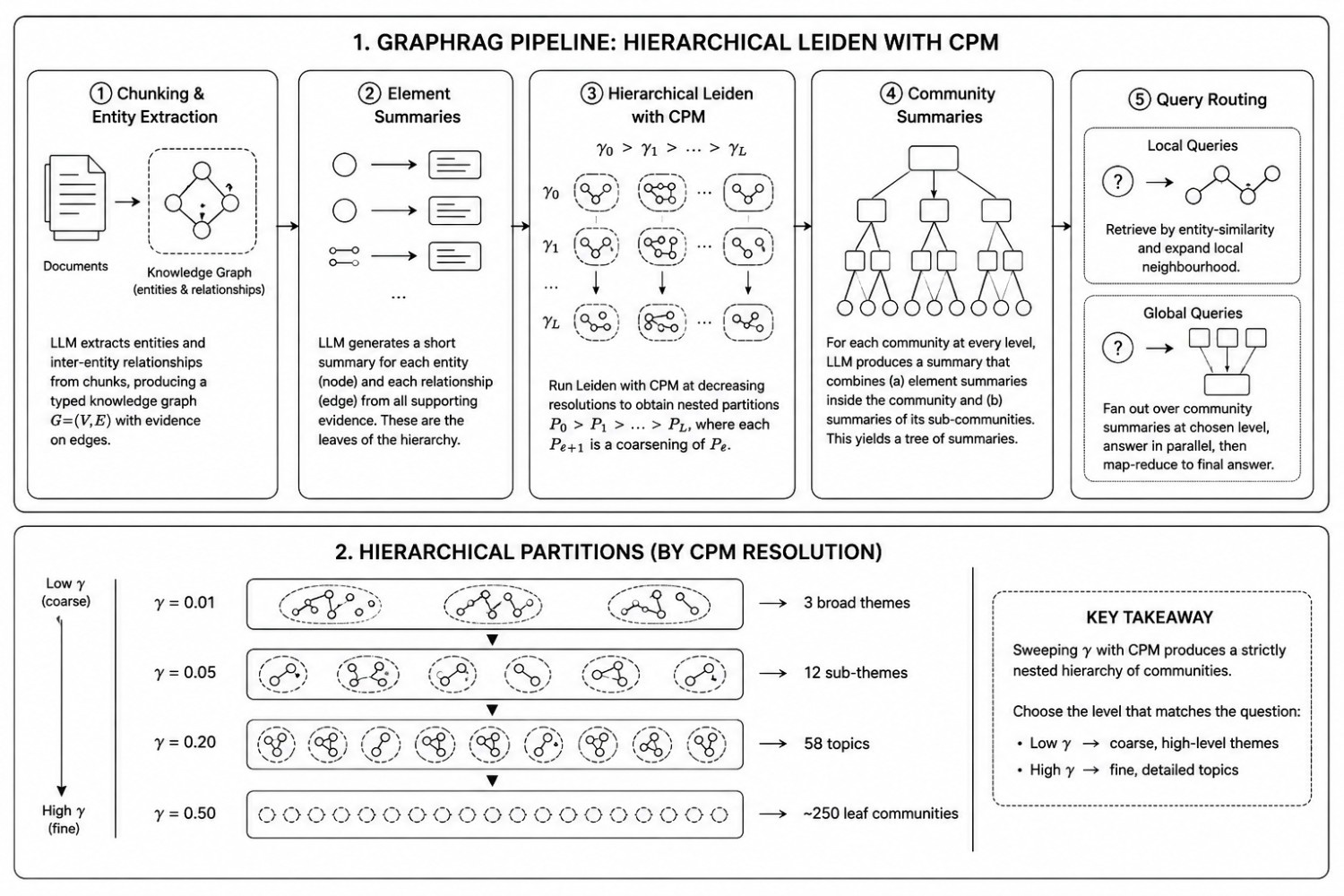

Limitations and Open Questions

1. Leiden is currently the strongest general-purpose community detection algorithm, but it is not perfect. Community detection itself is ill-defined: different objectives such as modularity and CPM can produce different yet equally reasonable partitions. Leiden is also stochastic, so different random seeds may produce different communities
2. More importantly, a partition with higher modularity does not always produce better retrieval or better LLM summaries. There is still no true end-to-end objective that optimizes clustering directly for GraphRAG quality.
3. CPM also introduces the resolution parameter $\gamma$, whose ideal value depends on the application. GraphRAG addresses this partly through hierarchical clustering, but query systems still need heuristics to decide which level of the hierarchy to use
4. Finally, not all semantic structure is community-shaped. Overlapping relationships, hub-and-spoke graphs, and bipartite structures are often poorly represented by strict partitions, making this an active area of ongoing research!

Appendix

1. Edge, D., Trinh, H., Cheng, N., Bradley, J., Chao, A., Mody, A., Truitt, S., Metropolitansky, D., Ness, R. O., & Larson, J. (2024). From Local to Global: A Graph RAG Approach to Query-Focused Summarization. Link
2. Gargi, U., Lu, W., Mirrokni, V., & Yoon, S. (2021). Large-Scale Community Detection on YouTube for Topic Discovery and Exploration. Proceedings of the International AAAI Conference on Web and Social Media, 5(1), 486-489 Link
3. Larson, J., & Truitt, S. (2024, February 13). GraphRAG: Unlocking LLM discovery on narrative private data. Microsoft Research Blog Link
4. Leskovec, J., & Krevl, A. (2014). SNAP Datasets: Stanford Large Network Dataset Collection - YouTube online social network. Stanford Network Analysis Platform Link
5. Splines. (n.d.). Modularity formula. Fast-Louvain Documentation Link
6. Traag, V. A., Waltman, L., & van Eck, N. J. (2019). From Louvain to Leiden: guaranteeing well-connected communities. Scientific Reports, 9(1) Link
7. Filippo Radicchi, Claudio Castellano, Federico Cecconi, Vittorio Loreto, and Domenico Parisi. Defining and identifying communities in networks. Physical Review E, 69(2), 2004 Link
8. Santo Fortunato and Marc Barthélemy. Resolution limit in community detection. Proceedings of the National Academy of Sciences (PNAS), 104(1):36–41, 2007 Link
9. Blondel, V. D., Guillaume, J.-L., Lambiotte, R., & Lefebvre, E. (2008). Fast unfolding of communities in large networks. Journal of Statistical Mechanics: Theory and Experiment, 2008(10), P10008. Link
10. Newman, M. E. J. (2006).Modularity and community structure in networks.Proceedings of the National Academy of Sciences, 103(23), 8577–8582. Link
11. Traag, V. A., Van Dooren, P., & Nesterov, Y. (2011). Narrow scope for resolution-limit-free community detection.Physical Review E, 84(1), 016114. Link
12. Canal NFS. (2024, November 26). Leiden algorithm explained: A smarter way to detect communities in networks Video
13. Splience. (2023, August 18). Discovering communities: Modularity & Louvain #SoMe3 Video
14. Microsoft Research. GraphRAG Research Appendix. GraphRAG. Available at Link
15. Reference figure1: Connected Papers website Screenshot Link
16. Diagrams and Artifacts used in the Blog: Figma File Link ### Suggested Reads
17. Fortunato, S., & Barthélemy, M. (2007). Resolution limit in community detection. PNAS 104(1): 36–41. https://doi.org/10.1073/pnas.0605965104
18. Traag, V. A., Van Dooren, P., & Nesterov, Y. (2011). Narrow scope for resolution-limit-free community detection. Physical Review E 84(1): 016114. https://doi.org/10.1103/PhysRevE.84.016114
19. Radicchi, F., Castellano, C., Cecconi, F., Loreto, V., & Parisi, D. (2004). Defining and identifying communities in networks. PNAS 101(9): 2658–2663. https://doi.org/10.1073/pnas.0400054101 — for the “weak community” definition you may want to cite when introducing the resolution limit.
20. The leidenalg Python package documentation, particularly the Advanced and Multiplex sections. https://leidenalg.readthedocs.io